The general form of NURBS is defined as:

, where N is the B-Spline basis function, n is the number of control points, $w_i$ are the weights, $P_i$ are control points, and k is the degree.

The B-Spline basis function of degree 0 is defined as:

For higher degrees, the B-Spline basis functions are defined recursively:

, where are knots, $k$ is the degree.

Surely, calculating this function when rendering every frame is horribly slow, but luckily, we're able to simplify this if we know what degree we want.

Cubic convolution provides a fast way to interpolate the texture data, which Keys originally proposed. With this method, texture sampling can be simplified to taking four samples, multiplying them with four weights, and adding all of them together. It takes discrete image data and an interpolation kernel and outputs continuous data. The convolution kernel is the following:

Where $a$ is a constant, we usually choose $-0.5$ as the value. To apply the above kernel, we use the following function:

Where $i$ is the index of the input image data, $c_{i}$ is the colour value, and $x$ is the interpolation point. Because $u(s)$ is $0$ if $s$ is not in the range of $[-2, 2]$, $x_i$ can only be the four nearest indexes to $x$.

For example, if $x$ is 5.5, then $x_i$ can only be $4$, $5$, $6$ and $7$, and the parameter $s$ of the kernel function $u(s)$ can only be $1.5$, $0.5$, $-0.5$ and $-1.5$. We then take the four pixels and multiply them by $u(s)$, resulting in:

In the last article, we discussed polynomial interpolation. It works, but we will struggle to find coefficients for big data sets. Instead of using polynomial interpolation, we can use splines to solve this issue.

Splines define multiple pieces of a curve and keep the curve smooth by ensuring the tangent of each point on the curve is continuous. Therefore, it does not need to increase the degree when we add more values to interpolate. This article is going to discuss some commonly used splines.

B-Spline Curves

The form of the B-Spline is defined recursively.

Where $n$ is the degree of the spline; $t$ is knots; $a$ is control points; $B$ is the B-spline basis function, defined by:

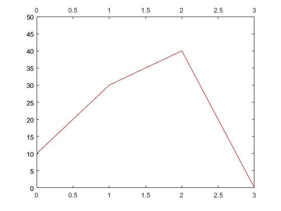
Interpolation is commonly used in computer programs. The most common interpolation method is linear interpolation, which takes two values and generates continuous uniform distributed results. For example, say we have a data set [10, 30, 40, 0]. The linear interpolation result of the data set will be like the following:

As the figure shows, linear interpolation does generate a continuous result. However, the curve that it generates could be smoother. Sometimes, we may not want those sharp corners. For example, if we're going to describe a spherical object, those sharp corners may make it look bad; Or if we are trying to interpolate an image, we may find the interpolated image weird.

To address this issue, we should use interpolation methods which generate smooth results.

Polynomial Interpolation

The data set [10, 30, 40, 0] contains four values, which means to describe a curve passing all four points, we need a three-degree polynomial, $ax^3+bx^2+cx+d=y$. Where $a$, $b$, $c$ and $d$ are coefficients, we will need to find them out. It is easy because with known $x$ and $y$ values, we can create a linear system based on them and use matrices to solve the issue.

The linear system based on the data set is:

And the matrix form of the above is:

The Image Distoration Issue and Anti-aliasing Algorithms

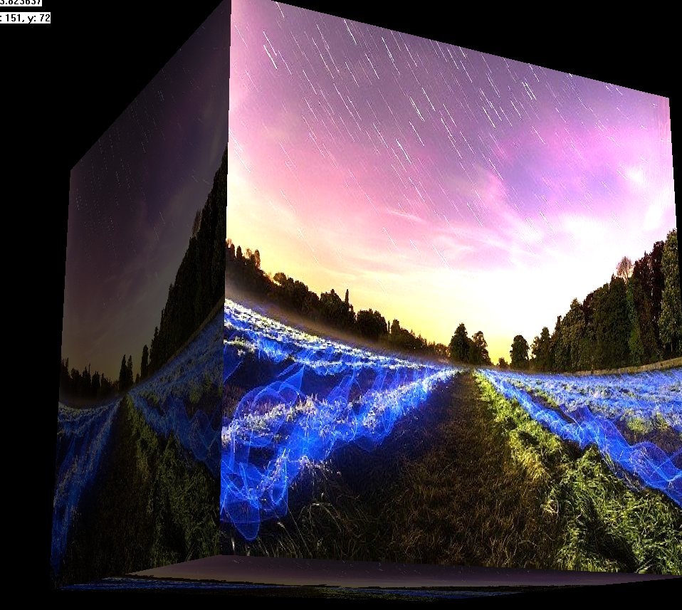
In 3D rendering, aliasing or image distortion is a difficult part that requires a lot of calculations to solve. It distorts images and makes images a bit ugly. For example, the following image was rendered by my SWRenderer project without any anti-aliasing:

The edges of the box are jagged.

Luckily, there are a few ways to tackle this issue. The simplest way is supersampling. It is to divide each pixel into multiple subpixels, render each subpixel and output the average value of the subpixels for each pixel. However, despite this method being able to solve the issue perfectly, it needs too much calculation and is almost impossible to use in realtime rendering. Instead, multisample is more commonly used.

The multisample algorithm only renders each pixel once, but it still gives an excellent result.

The Algorithm

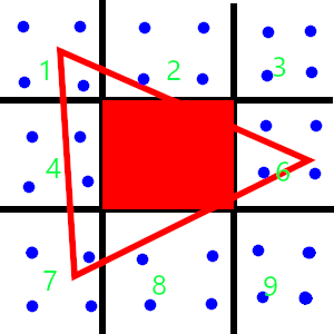
Say we are rendering a triangle like the above. The blue points are the subsamples, and the red triangle is the triangle we are rendering.

Without multisampling, the output image may look like the following, as only pixel 5 is fully covered by the triangle.

To make the image better, we divide pixels which are not fully covered by a triangle into a couple of subpixels. Instead of rendering them, we only use them to calculate the coverage of the pixel. If a pixel is fully covered, we deem the coverage of the pixel to be 100%.